
[논문리뷰] SAM-6D: Segment Anything Model Meets Zero-Shot 6D Object Pose Estimation (CVPR 2024)
SAM이 아무 물체나 분할할 수 있다면, 학습에 없던 물체의 6D pose도 zero-shot으로 구할 수 있지 않을까? SAM-6D는 이 질문을 “어디 있는가(segmentation)”와 “어떤 자세인가(pose)”의 두 단계로 나눠 답한다.
논문 정보
| 항목 | 내용 |
|---|---|
| 제목 | SAM-6D: Segment Anything Model Meets Zero-Shot 6D Object Pose Estimation |
| 저자 | Jiehong Lin, Lihua Liu, Dekun Lu, Kui Jia |
| 소속 / 연도 | DexForce · CUHK-Shenzhen · South China University of Technology, CVPR 2024 (arXiv:2311.15707) |
| 분야 | CV / zero-shot 6D object pose estimation |
| 코드 | GitHub |
1. Introduction
과제는 zero-shot 6D object pose estimation이다: 어질러진(cluttered) RGB-D 장면에서, 학습 때 본 적 없는 novel object를 찾아내고 그 6자유도 자세를 추정한다.
- instance-level 방법은 물체마다 학습 데이터가 필요하고, category-level 방법은 아는 카테고리 안에서만 일반화한다. 둘 다 novel object에는 못 미친다
- 마침 SAM(Segment Anything Model) 이 프롬프트 기반 분할에서 뛰어난 zero-shot 전이 성능을 보였다. 이를 novel object 탐지의 기반으로 삼는다
SAM-6D는 과제를 두 개의 전용 서브네트워크로 나눈다.
- ISM(Instance Segmentation Model): SAM으로 class-agnostic proposal을 만들고, 대상 물체와의 matching score로 걸러 novel object의 instance mask를 얻는다
- PEM(Pose Estimation Model): pose 추정을 proposal 점과 물체 모델 점 사이의 partial-to-partial point matching으로 정식화해 \((R, t)\) 를 구한다
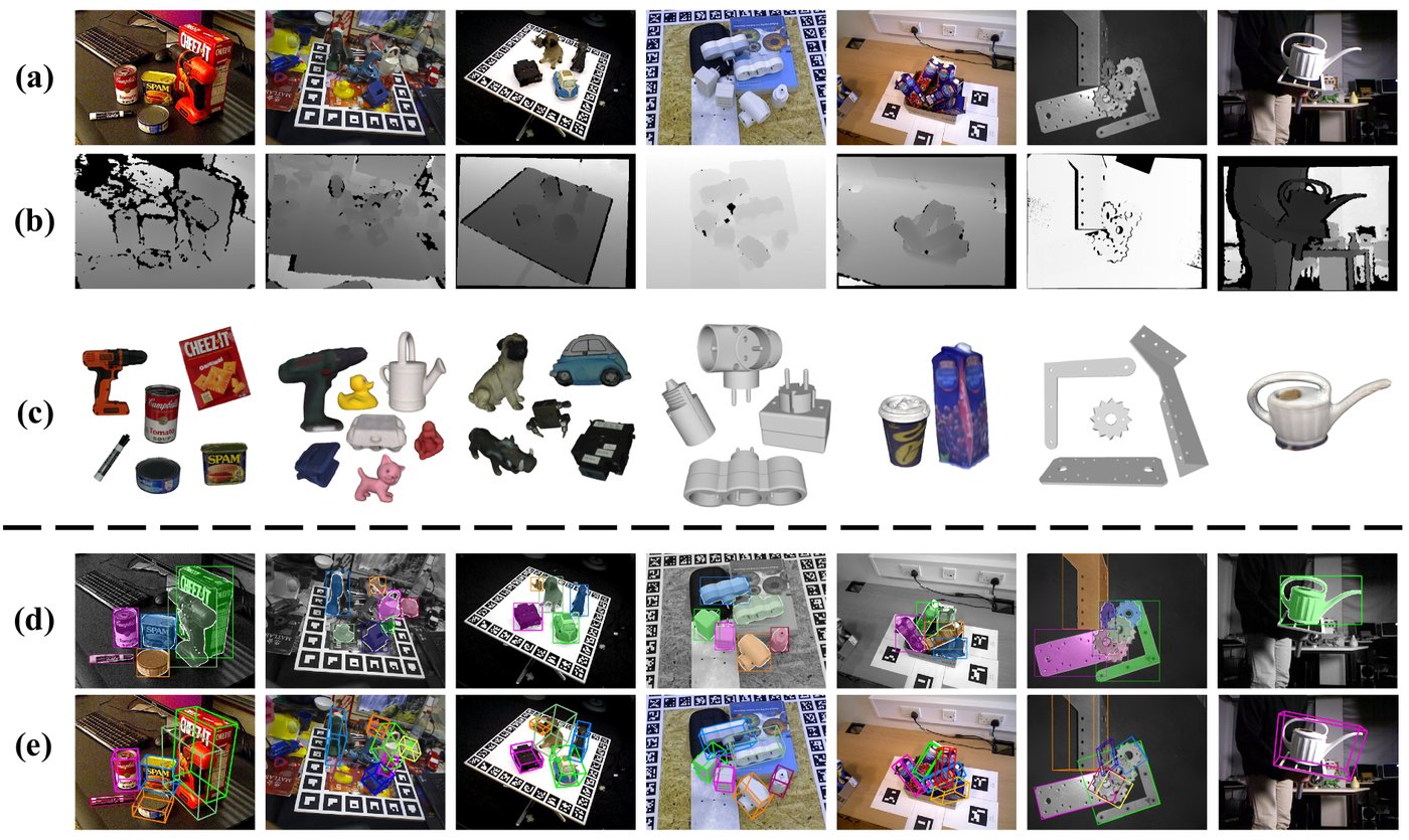 [Figure 1] cluttered RGB-D 장면(a, b)에서의 novel object 분할(c)과 6D pose 추정(d)
논문이 내세우는 기여는 다음과 같다.
- SAM 기반 ISM + point matching 기반 PEM의 SAM-6D framework
- semantic만이 아니라 semantic·appearance·geometric 세 항을 결합한 object matching score
- 대응 없는 점을 처리하는 background token 설계와 coarse → fine two-stage point matching
- dense 대응을 효율적으로 다루는 Sparse-to-Dense Point Transformer(SDPT)
2. Related Work
2.1 Segment Anything
SAM은 프롬프트(점·박스 등)를 받아 분할하는 foundation model로, 의료 영상·위장(camouflaged) 물체·3D 과제 등으로 응용이 확장됐다. novel object 탐지에 적용한 CNOS가 SAM-6D의 ISM과 가장 가까운 선행 연구다.
2.2 Pose Estimation of Novel Objects
novel object pose 추정은 크게 두 갈래다.
- image matching: 렌더링한 template과 입력을 이미지 수준에서 비교·검색 (MegaPose 등)
- feature matching: 2D-3D 또는 3D-3D 특징 대응을 만들어 pose를 푼다 (OnePose, ZeroPose 등)
SAM-6D는 feature matching 계열이며, optimal transport의 반복 최적화 없이 background token으로 partial 대응을 처리하는 점, two-stage로 대응을 정교화하는 점이 다르다.
3. SAM-6D 방법론
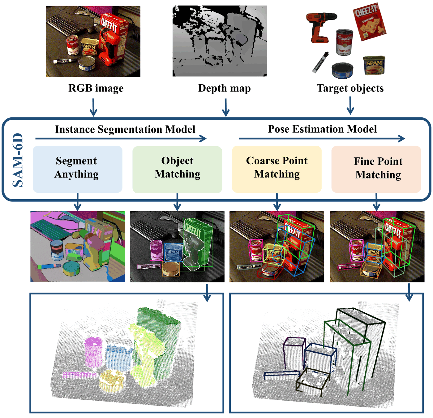 [Figure 2] ISM(위)과 PEM(아래)으로 구성된 전체 framework와 세 matching score 계산 과정
3.1 Instance Segmentation Model (ISM)
Proposal 생성. SAM은 이미지 인코더 \(\Phi_{\text{Image}}\), 프롬프트 인코더 \(\Phi_{\text{Prompt}}\), 마스크 디코더 \(\Psi_{\text{Mask}}\) 로 구성된다. 이미지 \(\mathcal{I}\) 와 프롬프트 \(\mathcal{P}_r\) 에 대해
\[\mathcal{M},\ \mathcal{C} = \Psi_{\text{Mask}}\!\left(\Phi_{\text{Image}}(\mathcal{I}),\ \Phi_{\text{Prompt}}(\mathcal{P}_r)\right)\]- \(\mathcal{M}\): 예측된 proposal(마스크)들, \(\mathcal{C}\): 각 proposal의 confidence
- 프롬프트로 이미지 전체에 균일 격자로 뿌린 2D 점을 넣어 class-agnostic proposal을 왕창 만들고, confidence 임계값과 NMS로 정리한다
Object matching score. 이 proposal들 중 어느 것이 대상 물체인지 골라야 한다. 대상 물체의 CAD 모델을 \(N_\mathcal{T}\) 개 시점에서 렌더링해 template \(\{\mathcal{T}_k\}\) 를 만들고, DINOv2(ViT)로 proposal crop과 template 각각에서 class embedding \(f^{cls}\) 와 patch embedding \(f^{patch}\) 를 뽑아 세 가지 점수를 계산한다.
① semantic matching score. proposal과 각 template의 class embedding 사이 cosine similarity를 구하고, 상위 \(K\) 개의 평균을 쓴다. similarity가 가장 높은 template을 \(\mathcal{T}_{best}\) 로 지정한다.
② appearance matching score. 의미는 비슷해도 생김새가 다른 물체를 거르기 위해, patch 수준에서 비교한다.
\[s_{appe} = \frac{1}{N^{patch}_{\mathcal{I}_m}} \sum_{j=1}^{N^{patch}_{\mathcal{I}_m}} \max_{i}\ \cos\!\left( f^{patch}_{\mathcal{I}_m, j},\ f^{patch}_{\mathcal{T}_{best}, i} \right)\]- \(f^{patch}_{\mathcal{I}_m, j}\): proposal crop \(\mathcal{I}_m\) 의 \(j\) 번째 patch embedding, \(f^{patch}_{\mathcal{T}_{best}, i}\): 최적 template의 \(i\) 번째 patch embedding
- proposal의 각 patch가 template에서 가장 닮은 patch와 얼마나 닮았는지를 전 patch에 대해 평균한 것
③ geometric matching score. \(\mathcal{T}_{best}\) 의 회전과 proposal 점들의 평균 위치로 대략의 pose를 만들어 물체를 이미지에 투영하고, 그 bounding box \(\mathcal{B}_o\) 와 proposal의 bounding box \(\mathcal{B}_m\) 의 IoU를 잰다.
\[s_{geo} = \frac{\mathcal{B}_m \cap \mathcal{B}_o}{\mathcal{B}_m \cup \mathcal{B}_o}\]세 점수는 가시 비율 \(r_{vis}\) (물체가 가려지지 않고 보이는 비율 추정치)로 가중해 결합한다.
\[s_m = \frac{s_{sem} + s_{appe} + r_{vis}\, s_{geo}}{2 + r_{vis}}\]- 가림이 심하면(\(r_{vis}\) 작음) bounding box 비교가 불안정하므로 \(s_{geo}\) 의 비중을 자동으로 낮추는 설계다
- 최종적으로 \(s_m\) 이 임계값 \(\delta_m\) 을 넘는 proposal만 대상 물체의 instance로 남긴다
3.2 Pose Estimation Model (PEM)
pose 추정을 점 매칭 문제로 정식화한다. proposal의 depth에서 샘플링한 점 집합 \(\mathcal{P}_m \in \mathbb{R}^{N_m \times 3}\) 과, template들에서 집계한 물체 점 집합 \(\mathcal{P}_o \in \mathbb{R}^{N_o \times 3}\) 사이의 대응을 찾으면 \((R, t)\) 가 나온다. 문제는 가림·분할 오류 때문에 양쪽 다 일부만 겹치는(partial-to-partial) 매칭이라는 점이다.
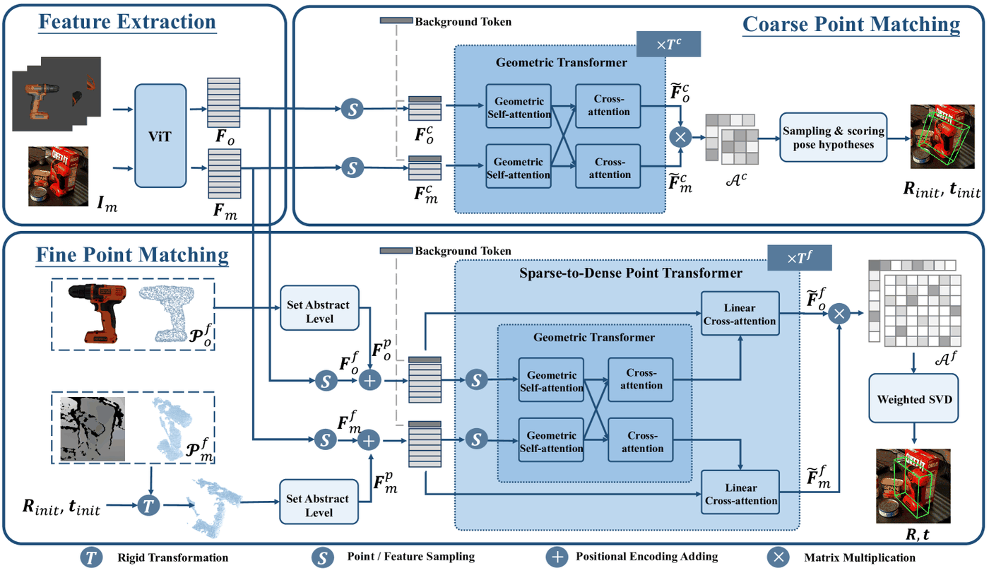 [Figure 3] PEM의 구조: Feature Extraction → Coarse Point Matching → Fine Point Matching
3.2.1 Feature Extraction
점을 3D 네트워크로 직접 인코딩하지 않고, DINOv2 ViT의 patch embedding을 픽셀 해상도로 보간해 각 3D 점에 부여한다. proposal 점 특징 \(F_m \in \mathbb{R}^{N_m \times C}\) 은 masked crop에서, 물체 점 특징 \(F_o \in \mathbb{R}^{N_o \times C}\) 는 여러 template의 가시 픽셀에서 집계한다 (\(C\): 특징 차원).
Background token. 대응이 없는 점을 다루기 위해 학습 가능한 token \(f^{bg}_m, f^{bg}_o \in \mathbb{R}^C\) 를 각 점 집합 앞에 붙인다. attention 행렬과 soft assignment는
\[\mathcal{A} = [\,f^{bg}_m,\ F_m\,]\,[\,f^{bg}_o,\ F_o\,]^\top \in \mathbb{R}^{(N_m+1)\times(N_o+1)}\] \[\tilde{\mathcal{A}} = \text{Softmax}_{\text{row}}(\mathcal{A}/\tau)\cdot\text{Softmax}_{\text{col}}(\mathcal{A}/\tau)\]- \(\mathcal{A}\) 의 첫 행·열이 background token 자리이고 나머지가 점끼리의 유사도다. \(\tau\): softmax 온도
- 행 방향·열 방향 softmax를 곱해 양방향으로 정규화된 soft assignment \(\tilde{\mathcal{A}}\) 를 만든다
- 각 proposal 점의 행에서 최댓값 위치가 0이면 대응 없음(background), 아니면 해당 물체 점과 매칭된다
- 매칭 쌍과 그 assignment 점수로 weighted SVD(Kabsch와 같은 닫힌형 풀이)를 돌려 \((R, t)\) 를 얻는다. optimal transport처럼 반복 최적화를 돌리지 않아도 된다는 것이 설계 포인트다
3.2.2 Coarse Point Matching
sparse한 점 집합(\(N^c_m = N^c_o = 196\))으로 초기 pose를 구한다.
- background token을 붙인 특징을 \(T^c\) 개의 Geometric Transformer(집합 내 self-attention + 집합 간 cross-attention)에 통과시킨다
- soft assignment \(\tilde{\mathcal{A}}^c\) 의 매칭 확률을 분포 삼아 점 삼중쌍(triplet)을 여러 번 샘플링해 pose 가설들을 만들고, 다음 점수로 평가한다
- \((R_{hyp}, t_{hyp})\): 평가할 pose 가설. 물체 점을 가설 pose의 역변환으로 proposal 좌표계에 되돌렸을 때, 각 proposal 점에서 가장 가까운 물체 점까지 거리의 평균이 분모다. 잘 맞는 가설일수록 \(s_{hyp}\) 가 크다
- 최고 점수 가설이 초기 pose \((R_{init}, t_{init})\) 가 된다
3.2.3 Fine Point Matching
dense한 점 집합(\(N^f_m = N^f_o = 2048\))으로 pose를 정밀화한다.
- 초기 pose 주입: proposal 점들을 \(R_{init}^\top(\mathcal{P}^f_m - t_{init})\) 로 미리 정렬해 두고, multi-scale Set Abstraction으로 만든 positional encoding을 특징에 더한다. coarse 단계의 대응 정보가 fine 단계의 시작점이 된다
- SDPT(Sparse-to-Dense Point Transformer): 2048점 전체에 일반 transformer를 쓰면 너무 비싸고, Linear Transformer는 모델링이 약하다. SDPT는 (1) dense 특징에서 sparse 부분집합을 뽑아 Geometric Transformer로 상호작용을 학습하고, (2) 그 결과를 Linear Cross-Attention(sparse가 key/value, dense가 query)으로 dense 전체에 전파한다. 이를 \(T^f\) 회 쌓는다
- 마지막 dense soft assignment에서 대응을 뽑아 weighted SVD로 최종 \((R, t)\) 를 계산한다
학습. PEM은 MegaPose가 공개한 대규모 합성 데이터(ShapeNet-Objects + Google-Scanned-Objects, 물체 약 5만 종·이미지 200만 장)로 학습한다. 두 단계의 attention 행렬을 InfoNCE contrastive loss로 감독하고, Adam으로 60만 iteration 학습한다. template은 학습 때 2개, 평가 때 42개를 쓴다.
4. Experiments
BOP benchmark의 7개 핵심 데이터셋(LM-O, T-LESS, TUD-L, IC-BIN, ITODD, HB, YCB-V)에서 평가한다. segmentation은 mAP(IoU 0.50~0.95), pose는 VSD·MSSD·MSPD 세 오차 지표의 평균 recall(AR)을 쓴다.
4.1 Instance Segmentation of Novel Objects
| Method | Seg. Model | \(s_{sem}\) | \(s_{appe}\) | \(s_{geo}\) | LM-O | T-LESS | TUD-L | IC-BIN | ITODD | HB | YCB-V | Mean |
|---|---|---|---|---|---|---|---|---|---|---|---|---|
| ZeroPose | SAM | - | - | - | 34.4 | 32.7 | 41.4 | 25.1 | 22.4 | 47.8 | 51.9 | 36.5 |
| CNOS | FastSAM | - | - | - | 39.7 | 37.4 | 48.0 | 27.0 | 25.4 | 51.1 | 59.9 | 41.2 |
| CNOS | SAM | - | - | - | 39.6 | 39.7 | 39.1 | 28.4 | 28.2 | 48.0 | 59.5 | 40.4 |
| SAM-6D | FastSAM | ✓ | ✗ | ✗ | 39.5 | 37.6 | 48.7 | 25.7 | 25.3 | 51.2 | 60.2 | 41.2 |
| SAM-6D | FastSAM | ✓ | ✓ | ✗ | 40.6 | 39.3 | 50.1 | 27.7 | 29.0 | 52.2 | 60.6 | 42.8 |
| SAM-6D | FastSAM | ✓ | ✗ | ✓ | 40.4 | 41.4 | 49.7 | 28.2 | 30.1 | 54.0 | 61.1 | 43.6 |
| SAM-6D | FastSAM | ✓ | ✓ | ✓ | 42.2 | 42.0 | 51.7 | 29.3 | 31.9 | 54.8 | 62.1 | 44.9 |
| SAM-6D | SAM | ✓ | ✗ | ✗ | 43.4 | 39.1 | 48.2 | 33.3 | 28.8 | 55.1 | 60.3 | 44.0 |
| SAM-6D | SAM | ✓ | ✓ | ✗ | 44.4 | 40.8 | 49.8 | 34.5 | 30.0 | 55.7 | 59.5 | 45.0 |
| SAM-6D | SAM | ✓ | ✗ | ✓ | 44.0 | 44.7 | 54.8 | 33.8 | 31.5 | 58.3 | 59.9 | 46.7 |
| SAM-6D | SAM | ✓ | ✓ | ✓ | 46.0 | 45.1 | 56.9 | 35.7 | 33.2 | 59.3 | 60.5 | 48.1 |
[Table 1] BOP 7개 데이터셋에서의 novel object instance segmentation 결과 (IoU 0.50~0.95의 mAP)
matching score를 하나씩 쌓아 보면(SAM 기준) semantic만 44.0 → appearance 추가 45.0 → geometric 추가 46.7 → 셋 결합 48.1로, 세 항이 각각 기여함을 보인다.
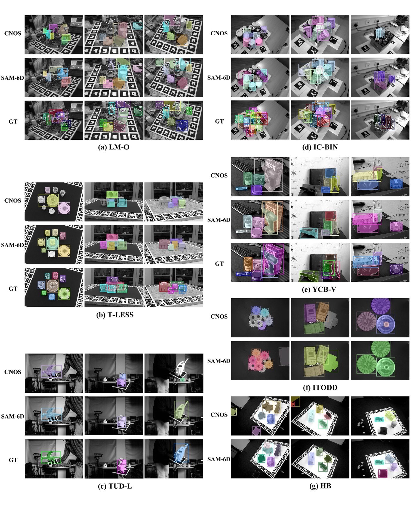 [Figure 6] BOP 7개 데이터셋에서의 novel object instance segmentation 정성 결과
4.2 Pose Estimation of Novel Objects
4.2.1 기존 방법과 비교
With Supervised Detection / Segmentation. MaskRCNN 검출(CosyPose 제공 마스크)을 쓰는 조건:
| Method | Input | LM-O | T-LESS | TUD-L | IC-BIN | ITODD | HB | YCB-V | Mean |
|---|---|---|---|---|---|---|---|---|---|
| MegaPose | RGB | 18.7 | 19.7 | 20.5 | 15.3 | 8.00 | 18.6 | 13.9 | 16.2 |
| MegaPose† | RGB | 53.7 | 62.2 | 58.4 | 43.6 | 30.1 | 72.9 | 60.4 | 54.5 |
| MegaPose† | RGB-D | 58.3 | 54.3 | 71.2 | 37.1 | 40.4 | 75.7 | 63.3 | 57.2 |
| ZeroPose | RGB-D | 26.1 | 24.3 | 61.1 | 24.7 | 26.4 | 38.2 | 29.5 | 32.6 |
| ZeroPose† | RGB-D | 56.2 | 53.3 | 87.2 | 41.8 | 43.6 | 68.2 | 58.4 | 58.4 |
| SAM-6D | RGB-D | 66.5 | 66.0 | 80.9 | 61.9 | 31.9 | 81.8 | 79.6 | 66.9 |
With Zero-Shot Detection / Segmentation:
| Method | Input | Detection / Seg. | LM-O | T-LESS | TUD-L | IC-BIN | ITODD | HB | YCB-V | Mean |
|---|---|---|---|---|---|---|---|---|---|---|
| ZeroPose | RGB-D | ZeroPose | 26.0 | 17.8 | 41.2 | 17.7 | 38.0 | 43.9 | 25.7 | 25.7 |
| ZeroPose† | RGB-D | ZeroPose | 49.1 | 34.0 | 74.5 | 39.0 | 42.9 | 61.0 | 57.7 | 51.2 |
| SAM-6D | RGB-D | ZeroPose | 63.5 | 43.0 | 80.2 | 51.8 | 48.4 | 69.1 | 79.2 | 62.2 |
| MegaPose* | RGB | CNOS (FastSAM) | 22.9 | 17.7 | 25.8 | 15.2 | 10.8 | 25.1 | 28.1 | 20.8 |
| MegaPose†* | RGB | CNOS (FastSAM) | 49.9 | 47.7 | 65.3 | 36.7 | 31.5 | 65.4 | 60.1 | 50.9 |
| MegaPose†* | RGB-D | CNOS (FastSAM) | 62.6 | 48.7 | 85.1 | 46.7 | 46.8 | 73.0 | 76.4 | 62.8 |
| ZeroPose†* | RGB-D | CNOS (FastSAM) | 53.8 | 40.0 | 83.5 | 39.2 | 52.1 | 65.3 | 65.3 | 57.0 |
| GigaPose | RGB | CNOS (FastSAM) | 29.9 | 27.3 | 30.2 | 23.1 | 18.8 | 34.8 | 29.0 | 27.6 |
| GigaPose† | RGB | CNOS (FastSAM) | 59.9 | 57.0 | 63.5 | 46.7 | 39.7 | 72.2 | 66.3 | 57.9 |
| SAM-6D | RGB-D | CNOS (FastSAM) | 65.1 | 47.9 | 82.5 | 49.7 | 56.2 | 73.8 | 81.5 | 65.3 |
| SAM-6D | RGB-D | SAM-6D (FastSAM) | 66.7 | 48.5 | 82.9 | 51.0 | 57.2 | 73.6 | 83.4 | 66.2 |
| SAM-6D | RGB-D | SAM-6D (SAM) | 69.9 | 51.5 | 90.4 | 58.8 | 60.2 | 77.6 | 84.5 | 70.4 |
[Table 2] BOP 7개 데이터셋에서의 novel object pose estimation 결과 (VSD·MSSD·MSPD의 평균 AR). † = MegaPose의 pose refinement 사용, * = BOP leaderboard 공개 결과
supervised 검출 조건에서도 SAM-6D(66.9)가 refinement를 쓴 ZeroPose†(58.4)·MegaPose†(57.2)를 앞서고, 자체 ISM의 zero-shot segmentation과 결합하면 70.4로 가장 높다. render-and-compare 방식의 무거운 refinement 없이 얻은 수치다.
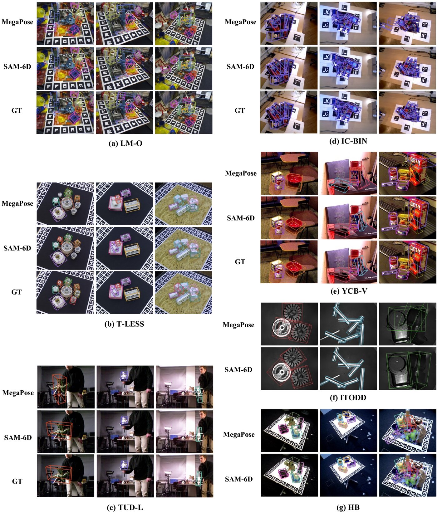 [Figure 10] BOP 7개 데이터셋에서의 novel object pose estimation 정성 결과
4.2.2 Ablation Studies and Analyses
Background token vs Optimal Transport. 더 정확하면서 3배 이상 빠르다.
| AR | Time (s) | |
|---|---|---|
| PEM with Optimal Transport | 81.4 | 4.31 |
| PEM with Background Tokens | 84.5 | 1.36 |
[Table 3] YCB-V에서 Optimal Transport와 background token 설계의 정확도·PEM 추론 시간 비교
Two-stage 전략. fine 단계는 초기화 없이는 동작하지 못하고, coarse만으로는 정밀도가 모자란다.
| Coarse Point Matching | Fine Point Matching | AR |
|---|---|---|
| ✓ | ✗ | 77.6 |
| ✗ | ✓ | 40.2 |
| ✓ | ✓ | 84.5 |
[Table 4] 두 point matching 단계 전략의 ablation (YCB-V)
Fine Point Matching의 transformer 종류. sparse의 표현력과 dense의 해상도를 결합한 효과.
| Transformer | #Point | AR |
|---|---|---|
| Geometric Transformer | 196 | 81.7 |
| Linear Transformer | 2048 | 78.4 |
| Sparse-to-Dense Point Transformer | 196 → 2048 | 84.5 |
[Table 5] Fine Point Matching에 쓰는 transformer 종류 비교 (YCB-V)
4.3 Runtime Analysis
RTX 3090 기준 이미지당 평균:
| Segmentation Model | Instance Segmentation | Pose Estimation | All |
|---|---|---|---|
| FastSAM | 0.45 | 0.98 | 1.43 |
| SAM | 2.80 | 1.57 | 4.37 |
[Table 6] segmentation model에 따른 이미지당 평균 runtime (초, RTX 3090)
5. Conclusion
SAM-6D는 zero-shot 6D pose estimation을 ISM과 PEM의 두 단계로 푸는 framework다. ISM은 SAM의 proposal을 semantic·appearance·geometric 세 matching score로 걸러 novel object를 분할하고, PEM은 background token 기반 two-stage point matching과 SDPT로 dense 대응을 만들어 pose를 계산한다. 저자들은 BOP 7개 데이터셋의 instance segmentation과 pose estimation 두 과제 모두에서 기존 방법을 능가했으며, 이것이 SAM-6D의 강한 일반화 능력을 보여준다고 결론짓는다.