
[논문리뷰] MapAnything: Universal Feed-Forward Metric 3D Reconstruction (3DV 2026)
12가지가 넘는 3D reconstruction 과제를 모델 하나, forward 한 번으로. MapAnything은 이미지 1~N장에 camera intrinsics·pose·depth 같은 geometric 입력을 선택적으로 더 받아, metric(실제 척도) 3D 장면 geometry와 카메라를 직접 회귀하는 통합 transformer다. 장면을 depth map·local ray map·camera pose·metric scale factor로 분해한 factored representation이 핵심이다. uncalibrated SfM부터 calibrated MVS, monocular depth, camera localization, depth completion까지 한 모델이 전문(specialist) 모델들과 대등하거나 앞선다.
논문 정보
| 항목 | 내용 |
|---|---|
| 제목 | MapAnything: Universal Feed-Forward Metric 3D Reconstruction |
| 저자 | Nikhil Keetha, Norman Müller, Johannes Schönberger, Lorenzo Porzi, Yuchen Zhang, Tobias Fischer, Arno Knapitsch, Duncan Zauss, Ethan Weber, Nelson Antunes, Jonathon Luiten, Manuel Lopez-Antequera, Samuel Rota Bulò, Christian Richardt, Deva Ramanan, Sebastian Scherer, Peter Kontschieder |
| 소속 / 연도 | Meta Reality Labs, Carnegie Mellon University, 3DV 2026 (arXiv:2509.13414) |
| 분야 | CV / metric 3D reconstruction, visual geometry |
| 코드 | GitHub |
1. Introduction
이미지 기반 3D reconstruction은 전통적으로 SfM(structure-from-motion), photometric stereo, shape-from-shading 등으로 풀어 왔다. 문제를 다루기 쉽게 만들기 위해 고전적 접근은 feature 검출·matching, two-view pose 추정, camera calibration·resectioning, rotation·translation averaging, bundle adjustment(BA), MVS(multi-view stereo), monocular surface 추정 같은 별개의 과제들로 분해했다. 최근 연구는 이 문제들을 feed-forward architecture로 통합해서 푸는 엄청난 잠재력을 보여 줬다.
기존 feed-forward 연구들이 과제들을 따로 다루거나 사용 가능한 입력 modality를 전부 활용하지 않은 반면, 이 논문은 다양한 3D reconstruction 과제를 위한 통합 end-to-end 모델을 제안한다. MapAnything은 가장 일반적인 uncalibrated SfM 문제뿐 아니라 calibrated SfM, multi-view stereo, monocular depth 추정, camera localization, metric depth completion 같은 하위 문제들의 다양한 조합을 풀 수 있다. 이런 통합 모델의 학습을 위해 (1) 가용한 geometric modality들을 지원하는 유연한 입력 scheme을 도입하고, (2) 이 다양한 과제 전부를 지원하는 적절한 출력 공간을 제안하며, (3) 유연한 데이터셋 통합·표준화를 논한다.
이 난제들을 해결하는 MapAnything의 핵심 통찰은 multi-view 장면 geometry의 factored representation이다. 장면을 pointmap의 모음으로 직접 표현하는 대신, depth map·local ray map·camera pose와 local 재구성을 전역적으로 일관된 metric 좌표계로 올려 주는 metric scale factor의 모음으로 표현한다. 이 factored representation을 출력과 (선택적) 입력 양쪽에 써서, 가용한 보조 geometric 입력을 활용할 수 있다. 예를 들어 robotics 응용은 camera intrinsics(ray)나 extrinsics(pose)를 알고 있는 경우가 많다. 또 이 표현의 큰 장점은 부분적 annotation만 있는 다양한 데이터셋(예: 비율만 맞는 “up-to-scale” geometry만 annotation된 데이터셋)으로도 효과적으로 학습할 수 있다는 것이다.
기여를 요약하면 다음과 같다.
- 통합 feed-forward 모델: 12가지가 넘는 문제 구성을 지원하는 multi-view metric 3D reconstruction 모델. end-to-end transformer가 개별 맞춤 모델들의 나이브한 집합보다 효율적으로 학습되고, 이미지 외에도 camera intrinsics·extrinsics·depth·metric scale factor 같은 선택적 geometric 정보를 활용
- factored scene representation: 분리된(decoupled) 입력과 효과적인 metric 3D reconstruction 예측을 유연하게 가능케 하는 표현. 중복이나 비싼 후처리 없이 multi-view 픽셀별 장면 geometry와 카메라를 직접 계산
- state-of-the-art 성능: 다른 feed-forward 모델들과 비교해, 특정 과제 전용으로 만든 expert 모델들과 대등하거나 능가
- 오픈소스 공개: 데이터 처리·inference·벤치마크·학습·ablation 코드와 Apache 2.0 라이선스의 사전학습 모델 공개
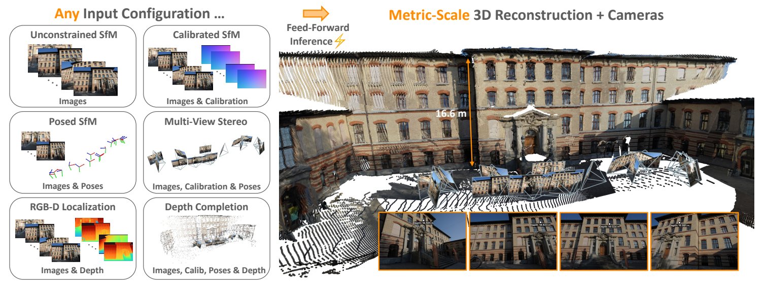 [Figure 1] 이미지 N장과 선택적 camera pose·intrinsics·depth map으로부터 metric 3D reconstruction과 카메라 정보를 예측하는 유연한 통합 feed-forward 모델 MapAnything. camera localization·SfM·MVS·metric depth completion 등 12가지 이상의 과제 지원
2. Related Work
Towards Universal 3D Reconstruction. 별개의 reconstruction 과제마다 특화 방법을 설계하는 전통적 접근과 달리, 최근 연구들은 단일 feed-forward architecture로 과제들을 함께 푸는 데서 큰 가능성을 보였다. DeMoN·DeepTAM·DeepV2D 같은 초기 연구가 CNN으로 이 방향을 탐구했지만 고전적 expert 모델의 성능에 미치지 못했다. 딥러닝의 발전에 힘입어 PF-LRM, RayDiffusion, DUSt3R, VGGSfM, VGGT 같은 최근 방법들은 대량의 데이터로 transformer를 scale up했다. 이 돌파구에도 불구하고 이 방법들은 여전히 고정된 입출력 modality의 3D reconstruction 과제 일부에 국한되거나, view 수가 적거나 고정돼 있거나, 비교적 제한된(주로 object 중심) 시나리오에서만 잘 동작한다. MapAnything은 임의 개수의 입력 view에 대해 이질적인 입출력 modality를 지원하는, geometry에 근거한 유연한 architecture 설계로 이 한계를 넘는다.
Multi-View Feed-forward Reconstruction. DUSt3R와 그 metric 후속작 MASt3R는 결합된(coupled) 장면 표현을 예측한다. 즉 카메라·pose·geometry가 pointmap 하나로 parameterize돼 사후에 복원해야 하고, multi-view unconstrained SfM을 하려면 비싼 후처리와 대칭 inference가 필요하다. 후속 연구들은 MASt3R 출력을 고전적 SfM·SLAM pipeline에 더 원칙적으로 통합했다. Spann3R·CUT3R·MUSt3R 같은 최근 연구는 transformer의 latent 상태 메모리로 고전적 최적화 없이 multi-view reconstruction을 가능하게 했지만, MASt3R의 two-view 출력에 전통적 최적화를 적용한 것의 성능에는 아직 미치지 못한다.
최근 MV-DUSt3R+와 VGGT는 DUSt3R architecture를 확장해 multi-view inference를 보였다. Reloc3r는 camera re-localization에 집중해 multi-view camera pose를 직접 예측한다. MV-DUSt3R+는 서로 다른 기준 view를 지원하도록 cross-attention transformer를 병렬화해 계산이 크게 늘었고, VGGT는 alternating attention transformer로 multi-view pointmap·depth·pose·tracking feature를 예측한다. FASt3R는 LLM의 long-sequence positional encoding을 써서 적은 view로 학습한 global attention을 더 많은 view에 적용한다. 최근의 \(\pi^3\) 는 VGGT를 fine-tuning해 첫 입력 프레임을 기준 좌표계로 쓰는 것을 없앴다. MV-DUSt3R+와 FASt3R 모두 예측이 결합된 장면 표현이라 이질적 입력을 다룰 수 없다. FASt3R가 보였듯 multi-view 설정에서 dense geometry 예측 능력은 보이지 않는 view들에 걸친 pose 추정에 영향을 받고, 이를 완화하려 FASt3R는 global·local pointmap 예측에 전용 DPT head를 둬 모든 view의 중복된 pointmap을 예측한다. VGGT도 pointmap용과 camera·depth용 두 branch로 여러 중복된 값을 예측한다. 동시 연구 \(\pi^3\) 는 up-to-scale로 분리된 local pointmap과 global pose를 예측해 이 중복을 없앴지만, 이 논문은 그 설계가 차선임을 발견한다(Table 5(a)). 반면 MapAnything은 완전히 factored된 표현, 즉 모든 view의 local ray 방향·ray를 따른 depth·global camera pose와 장면 전체의 단일 metric scale factor를 직접 예측한다. 이 정식화에서 ray 방향 예측(camera calibration에 해당)과 ray 기준 depth 추정은 view별 과제라 단일 dense prediction head로 예측할 수 있다. 기존 연구들이 unconstrained multi-view inference와 대규모 학습의 길을 닦았지만 모두 이미지 입력과 단순 pinhole 카메라 모델에 제한된 반면, MapAnything은 이질적 입력과 유연한 카메라 모델로 여러 view의 다양한 3D reconstruction·calibration 과제를 지원한다.
Geometry as Inputs or Conditioning. ray 방향·원점·depth map 같은 값들은 novel view synthesis, diffusion 기반 이미지 생성, 동적 비디오 depth 추정, 3D object shape completion의 conditioning 입력으로 탐구돼 왔다. Taskonomy는 vision 과제 성능 향상을 위한 multi-task 학습의 이득을 탐구했고, MultiMAE는 이 통찰 위에 이질적 입력의 유연한 조합을 지원하는 auto-encoder를 고안했지만 3D reconstruction 과제에는 적합하지 않다. Pow3R는 알려진 prior를 feed-forward 3D reconstruction의 입력으로 통합한 첫 연구지만, 초점거리 하나와 중심 principal point를 가진 pinhole 카메라 이미지 두 장만 지원하고, DUSt3R 위에 만들어져 metric scale 정보로 condition할 수 없다. 반면 MapAnything은 임의 개수의 입력 view와, metric scale과 중심 투영(central projection) 모델의 어떤 카메라든 지원하는 유연한 입력 parameterization을 갖는다.
3. MapAnything
MapAnything은 \(N\) 장의 RGB 이미지 \(\hat{\mathcal{I}} = (\hat{I}_i)_{i=1}^{N}\) 과, 전체 또는 일부 입력 view에 대한 선택적 geometric 입력을 받는 end-to-end 모델이다. geometric 입력은 (a) ray 방향으로 표현한 일반적인 중심 카메라 calibration \(\hat{\mathcal{R}} = (\hat{R}_i)_{i \in S_{\text{r}}}\), (b) 첫 view \(\hat{I}_1\) 좌표계의 pose(quaternion \(\hat{\mathcal{Q}} = (\hat{Q}_i)_{i \in S_{\text{q}}}\) 와 translation \(\hat{\mathcal{T}} = (\hat{T}_i)_{i \in S_{\text{t}}}\)), (c) 픽셀별 ray depth \(\hat{\mathcal{D}} = (\hat{D}_i)_{i \in S_{\text{d}}}\) 다. 여기서 \(S_{\text{r}}, S_{\text{q}}, S_{\text{t}}, S_{\text{d}}\) 는 프레임 index \([1, N]\) 의 부분집합이다. MapAnything은 이 입력들을 \(N\)-view factored metric 3D 출력으로 mapping한다.
\[f_{\text{MapAnything}}\big( \hat{\mathcal{I}}, [\hat{\mathcal{R}}, \hat{\mathcal{Q}}, \hat{\mathcal{T}}, \hat{\mathcal{D}}] \big) = \{ m, (R_i, \tilde{D}_i, \tilde{P}_i)_{i=1}^{N} \}\]여기서 \(m \in \mathbb{R}\) 은 예측된 전역 metric scale factor이고, 각 view \(i\) 에 대해 \(R_i \in \mathbb{R}^{3 \times H \times W}\) 는 예측된 local ray 방향, \(\tilde{D}_i \in \mathbb{R}^{1 \times H \times W}\) 는 up-to-scale 공간의 ray depth(tilde가 up-to-scale임을 나타낸다), \(\tilde{P}_i \in \mathbb{R}^{4 \times 4}\) 는 이미지 \(\hat{I}_1\) 좌표계에서 본 이미지 \(\hat{I}_i\) 의 pose로 quaternion \(Q_i\) 와 up-to-scale translation \(\tilde{T}_i \in \mathbb{R}^3\) 로 표현된다. 이 factored 출력으로 up-to-scale local pointmap(각 픽셀에 대응하는 3D 점)을 \(\tilde{L}_i = R_i \cdot \tilde{D}_i \in \mathbb{R}^{3 \times H \times W}\) 로 얻는다. 그리고 \(Q_i\) 에서 얻은 rotation 행렬 \(O_i\) 와 up-to-scale translation으로 world 좌표계의 \(N\)-view up-to-scale pointmap을 \(\tilde{X}_i = O_i \cdot \tilde{L}_i + \tilde{T}_i\) 로 계산한다. 최종적으로 \(N\) 개 입력 view의 metric 3D reconstruction(\(I_1\) 좌표계)은 \(X^{\text{metric}}_i = m \cdot \tilde{X}_i\) 다.
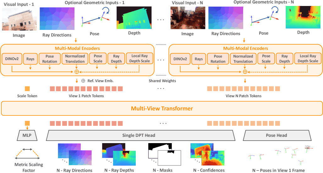 [Figure 2] N개의 시각·geometric 입력을 공통 latent 공간으로 인코딩해 합치고, 기준 view embedding과 scale token을 더해 multi-view alternating-attention transformer로 처리한 뒤 factored representation(ray·depth·pose·metric scale)을 예측하는 MapAnything architecture
3.1 Encoding Images & Geometric Inputs
\(N\) 개의 시각 입력과 선택적 dense geometric 입력을 먼저 공통 latent 공간으로 인코딩한다. 이미지는 DINOv2를 쓴다. CroCov2, DUSt3R의 image encoder, RADIO, 무작위 초기화 linear patchification 등 다양한 사전학습 선택지 중 DINOv2가 downstream 성능·수렴 속도·일반화(특히 작은 learning rate로 fine-tuning할 때) 면에서 최적이었다. DINOv2 ViT-G의 24번째 layer의 정규화된 patch feature \(F_{\text{I}} \in \mathbb{R}^{1536 \times H/14 \times W/14}\) 를 쓴다.
다른 geometric 값들도 인코딩할 수 있다. 네트워크에 넣기 전에 metric과 up-to-scale 값 모두에서 학습·inference가 가능하도록 factorize한다. rotation이나 translation만 따로 있는 경우(예: IMU·GPS prior)를 지원하고 translation과 scale의 얽힘을 다루기 위해 rotation과 translation을 분리해 인코딩한다. 또 depth와 pose가 항상 함께 입력된다고 가정하지 않으므로 둘의 정규화를 분리한다(예측 depth·pose를 함께 정규화하는 학습 목적함수와는 별개다. 거기서는 multi-view 일관성이 필요하다). 구체적으로 ray depth가 입력되면 먼저 view별 평균 depth \(\hat{z}_{di} \in \mathbb{R}^+\) 와 정규화된 ray depth \(\hat{D}_i / \hat{z}_{di}\) 로 분리한다. translation \(\hat{\mathcal{T}}\) 가 입력되면 world 좌표계까지의 평균 거리로 pose scale \(\hat{z}_{\text{p}} = \frac{1}{\lvert S_{\text{t}} \rvert} \sum_{i \in S_{\text{t}}} \| \hat{T}_i \|\) 를 계산한다(\(\lvert S_{\text{t}} \rvert\) 는 translation이 주어진 프레임 수). 이 pose scale은 translation이 입력된 모든 프레임에 같은 입력으로 쓰이고 정규화된 translation \(\hat{T}_i / \hat{z}_{\text{p}}\) 를 얻는 데도 쓰인다. geometric 입력의 metric scale 정보를 효과적으로 활용하는 것이 목적이므로, 특정 프레임의 pose·depth가 metric일 때만 pose scale·depth scale을 쓴다. metric scale 값은 크고 장면 크기에 따라 급격히 변하므로 인코딩 전에 log 변환한다.
ray 방향과 정규화된 ray depth는 얕은 convolutional encoder로 인코딩하는데, 공간 크기 변경은 크기 14의 pixel unshuffle 한 번으로만 일어난다. 이것이 dense geometric 입력을 DINOv2 feature와 같은 공간·latent 차원 \(F_{\text{R}}, F_{\text{D}} \in \mathbb{R}^{1536 \times H/14 \times W/14}\) 로 투영한다. 전역 non-pixel 값들, 즉 rotation(unit quaternion)·translation 방향·depth scale·pose scale은 GeLU 활성의 4-layer MLP로 \(F_{\text{Q}}, F_{\text{T}}, F_{\hat{z}_d}, F_{\hat{z}_{\text{p}}} \in \mathbb{R}^{1536}\) 로 투영한다. 모든 입력 값을 인코딩한 뒤 layer normalization을 거쳐 합산하고 다시 layer normalization해 view별 최종 인코딩을 얻고, 이를 token \(F_{\text{E}} \in \mathbb{R}^{1536 \times (HW/256)}\) 으로 펼친다.
\(N\) 개 view patch token에 학습 가능한 scale token 하나를 덧붙이고, 여러 view의 정보가 서로 attend·전파되도록 multi-view transformer에 넣는다. VGGT의 alternating-attention transformer 16 layer(24-head attention, latent 차원 1536, MLP 비율 4)를 쓰고 DINOv2 ViT-G의 마지막 16개 layer로 초기화한다. 기준 view(첫 번째)를 구별하기 위해 view \(I_1\) 의 patch token들에 상수 기준 view embedding을 더한다. 단순함을 위해 RoPE(Rotary Positional Embedding)는 쓰지 않는다. DINOv2의 patch 수준 positional encoding으로 충분하고, RoPE는 원래 모든 attention layer에 적용됐던 것이라 불필요한 bias를 들여온다.
3.2 Factored Scene Representation Prediction
multi-view transformer가 여러 view의 정보를 융합해 \(N\)-view patch token과 scale token을 출력하면, 이를 metric 3D geometry를 나타내는 factored 값들로 decode한다. DPT head로 \(N\)-view patch token을 \(N\) 개의 view별 dense 출력, 즉 ray 방향 \(R_i\)(단위 길이로 정규화), up-to-scale ray depth \(\tilde{D}_i\), depth의 비모호(non-ambiguous) class를 나타내는 mask \(M_i\), world 좌표계 pointmap confidence map \(C_i\) 로 decode한다. 또 \(N\)-view patch token을 average pooling 기반 convolutional pose head에 넣어 unit quaternion \(Q_i\) 와 up-to-scale translation \(\tilde{T}_i\) 를 예측한다. 마지막으로 scale token은 ReLU 활성의 2-layer MLP를 거쳐 metric scale factor를 예측하는데, 장면의 metric scale이 크게 변할 수 있어 예측을 지수적으로 scale해 \(m\) 을 얻는다. Table 5(a)에서 보듯 이 scale 예측의 분리(decoupling)가 universal metric feed-forward inference의 핵심이다. 이 factored 예측들을 합쳐 metric 3D reconstruction을 얻는다.
3.3 Training Universal Metric 3D Reconstruction
가용한 supervision에 따라 여러 loss로 end-to-end 학습한다. ray 방향 \(R_i\) 와 pose quaternion \(Q_i\) 는 장면 scale에 무관하므로 loss는 다음과 같다.
\[\mathcal{L}_{\text{rays}} = \sum_{i=1}^{N} \| \hat{R}_i - R_i \|, \quad \mathcal{L}_{\text{rot}} = \sum_{i=1}^{N} \min( \| \hat{Q}_i - Q_i \|, \ \| -\hat{Q}_i - Q_i \| )\]rotation loss의 \(\min\) 은 unit quaternion의 2대1 대응(\(\hat{Q}\) 와 \(-\hat{Q}\) 가 같은 rotation)을 고려한 것으로, 이 regression loss는 geodesic 각거리와 비슷하게 동작한다.
예측된 up-to-scale ray depth \(\tilde{D}_i\), translation \(\tilde{T}_i\), local pointmap \(\tilde{L}_i\), world 좌표계 pointmap \(\tilde{X}_i\) 에 대해서는 DUSt3R를 따라 ground-truth 유효 mask \(V_i\) 로 scaling factor를 계산한다. ground truth의 norm scale은 \(\hat{z} = \| (\hat{X}_i[V_i])_{i=1}^{N} \| / \sum_{i=1}^{N} V_i\)(유효 픽셀의 평균 norm), up-to-scale 예측의 norm scale은 \(\tilde{z} = \| (\tilde{X}_i[V_i])_{i=1}^{N} \| / \sum_{i=1}^{N} V_i\) 다. scale loss의 gradient가 geometry에 영향을 주지 않도록, 예측 metric scale factor \(m\) 과 gradient를 끊은(stop-grad, \(\mathrm{sg}\)) up-to-scale norm scale로 metric norm scale \(z^{\text{metric}} = m \cdot \mathrm{sg}(\tilde{z})\) 를 계산한다.
이 scaling factor들로 scale 불변 translation loss를 \(\mathcal{L}_{\text{translation}} = \sum_{i=1}^{N} \| \hat{T}_i / \hat{z} - \tilde{T}_i / \tilde{z} \|\) 로 계산한다. ray depth·pointmap·metric scale factor에는 log 공간에서 loss를 적용하는 것이 결정적이었다. 구체적으로 \(f_{\mathrm{log}}: \mathbf{x} \mapsto (\mathbf{x} / \|\mathbf{x}\|) \cdot \log(1 + \|\mathbf{x}\|)\) (방향은 유지하고 크기만 log로 압축하는 변환)를 쓴다. ray depth loss는
\[\mathcal{L}_{\text{depth}} = \sum_{i=1}^{N} \| f_{\mathrm{log}}(\hat{D}_i / \hat{z}) - f_{\mathrm{log}}(\tilde{D}_i / \tilde{z}) \|\]이고, local pointmap loss \(\mathcal{L}_{\text{lpm}}\) 도 \(\hat{L}_i / \hat{z}\) 와 \(\tilde{L}_i / \tilde{z}\) 로 같은 형태다. 학습 데이터의 결함과 outlier를 무시하기 위해 픽셀별 loss 상위 5%는 제외한다. DUSt3R처럼 confidence 가중 pointmap loss
\[\mathcal{L}_{\text{pointmap}} = \sum_{i=1}^{N} \big( C_i \| f_{\mathrm{log}}(\hat{X}_i / \hat{z}) - f_{\mathrm{log}}(\tilde{X}_i / \tilde{z}) \| - \alpha \log(C_i) \big)\]를 더한다(\(C_i\) 는 예측 confidence, \(-\alpha \log(C_i)\) 는 confidence를 무한정 낮추는 것을 막는 항). factored metric scale loss는 \(\mathcal{L}_{\text{scale}} = \| f_{\mathrm{log}}(\hat{z}) - f_{\mathrm{log}}(z^{\text{metric}}) \|\) 다. 미세한 디테일을 잡기 위해 local pointmap에 normal loss \(\mathcal{L}_{\text{normal}}\) 과, local pointmap의 \(z\)-depth log에 multi-scale gradient matching loss \(\mathcal{L}_{\text{GM}}\) 도 쓴다. 실사 데이터셋의 geometry는 거칠고 노이즈가 있어 이 두 loss는 synthetic 데이터셋에만 적용한다. 예측 mask에는 binary cross entropy loss \(\mathcal{L}_{\text{mask}}\) 를 쓴다. 전체 loss는 다음과 같다.
\[\mathcal{L} = 10 \cdot \mathcal{L}_{\text{pointmap}} + \mathcal{L}_{\text{rays}} + \mathcal{L}_{\text{rot}} + \mathcal{L}_{\text{translation}} + \mathcal{L}_{\text{depth}} + \mathcal{L}_{\text{lpm}} + \mathcal{L}_{\text{scale}} + \mathcal{L}_{\text{normal}} + \mathcal{L}_{\text{GM}} + 0.1 \cdot \mathcal{L}_{\text{mask}}\]factored 예측에는 global pointmap loss를 키우고 mask loss를 줄이는 것이 유리했다. 모든 regression loss에는 outlier robustness를 위한 adaptive robust loss(파라미터 \(c = 0.05\), \(\alpha = 0.5\))를 쓴다.
Training for Image & Geometric Inputs. 다양한 입력 구성을 지원하는 universal 모델을 한 번에 학습하기 위해, 학습 중 geometric 입력을 확률적으로 제공한다. 전체 geometric 입력 확률은 0.9이고, 각 factorization(ray 방향·ray depth·pose)의 입력 확률은 각 0.5다. depth가 선택되면 dense depth와 90% 무작위 sparsify된 depth가 같은 확률로 제공된다. 어느 view에 geometric 정보가 있는지에 대한 robustness와 유연성을 위해 view별 입력 확률 0.95를 쓰고, metric scale ground truth가 있는 데이터셋에서도 0.05의 확률로 metric scale factor를 입력하지 않는다.
Datasets. 실내·실외·in-the-wild를 아우르는 고품질 데이터셋 13개로 학습한다(Table 1). ScanNet++ v2와 TartanAirV2-WB는 train/validation/held-out test로, 나머지는 train/validation으로 나눈다. MPSD는 원래 monocular metric depth 데이터셋이지만 pose·camera 정보를 확보해 약 72K 장면의 실세계 multi-view metric scale 데이터셋으로 만들었고 이 metadata를 공개했다. 사전학습 모델 두 가지를 공개한다. 6개 데이터셋으로 학습한 Apache 2.0 모델과, 7개를 추가해 13개로 학습한 CC BY-NC 4.0 모델이다.
| Dataset | License | # Scenes | Metric |
|---|---|---|---|
| BlendedMVS | CC BY 4.0 | 493 | ✗ |
| Mapillary Planet-Scale Depth | CC BY-NC-SA | 71,428 | ✓ |
| ScanNet++ v2 | Non-commercial | 926 | ✓ |
| Spring | CC BY 4.0 | 37 | ✓ |
| TartanAirV2-WB | CC BY 4.0 | 49 | ✓ |
| UnrealStereo4K | MIT | 9 | ✓ |
| CC BY-NC 모델에 추가 사용: | |||
| Aria Synthetic Environments | Non-commercial | 103,890 | ✓ |
| DL3DV-10K | CC BY-NC 4.0 | 10,109 | ✗ |
| Dynamic Replica | Non-commercial | 523 | ✓ |
| MegaDepth | CC BY 4.0 | 269 | ✗ |
| MVS-Synth | Non-commercial | 120 | ✓ |
| ParallelDomain-4D | Non-commercial | 1,528 | ✓ |
| SAIL-VOS 3D | Non-commercial | 171 | ✓ |
| dense up-to-N-view 벤치마크용 held-out 장면: | |||
| ETH3D | CC BY-NC-SA 4.0 | 13 | ✓ |
| ScanNet++ v2 | Non-commercial | 30 | ✓ |
| TartanAirV2-WB | CC BY 4.0 | 5 | ✓ |
[Table 1] MapAnything의 학습·테스트에 쓴 데이터셋
Multi-View Sampling. 데이터셋마다 ground-truth depth·pose 기반 reprojection 오차 검사로 장면 안 모든 이미지의 pairwise covisibility를 미리 계산한다. 학습 중에는 covisibility threshold 25%로 random walk sampling을 수행해, 커버리지와 상호 정보량이 다양한 covisible view들의 단일 연결 그래프를 sampling한다.
4. Benchmarking & Results
넓은 범위의 3D vision 과제에서 MapAnything을 벤치마크한다. 과제마다 그 과제 전용으로 설계·학습된 expert baseline들과 비교하고, 모든 실험은 고정 seed로 수행한다.
Multi-View Dense Reconstruction. undistort된 ETH3D, ScanNet++ v2, TartanAirV2-WB에서 pointmap·pose·depth·ray 방향 추정 성능을 벤치마크한다. test 장면마다 미리 계산한 pairwise covisibility 기반으로 단일 연결 그래프를 이루는 최대 \(N\) 개 view를 무작위 sampling한다(입력에 서로 분리된 이미지 집합이 생기는 것을 막는다). Figure 4에서 보듯 MapAnything은 이미지 입력만으로도 VGGT를 포함한 다른 baseline들을 넘는 state-of-the-art dense multi-view reconstruction 성능을 보인다. 나아가 보조 geometric 입력을 feed-forward inference에 활용하면 재구성 성능이 큰 폭으로 더 오른다. 또 장면 prior를 활용하도록 설계된 two-view baseline인 Pow3R의 bundle adjustment 변형보다도 좋다. 이미지만 입력해도 재구성 출력의 충실도가 높다(Figure 3).
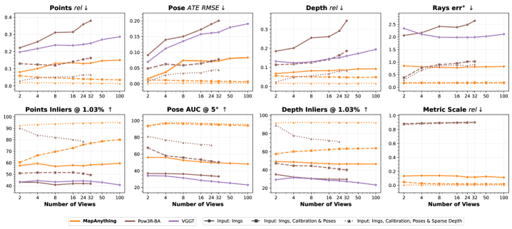 [Figure 4] 2~100개 입력 view와 다양한 입력 구성에서 state-of-the-art dense multi-view reconstruction 성능. ETH3D·ScanNet++ v2·TartanAirV2-WB 평균의 절대 상대 오차(rel), 상대 threshold 1.03에서의 inlier 비율(τ), 평균 정렬 궤적 오차(ATE RMSE), 오차 threshold 5°의 AUC(AUC@5), 평균 각오차(err°)
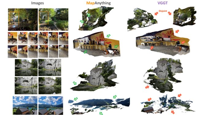 [Figure 3] in-the-wild 이미지만 입력한 VGGT와의 정성 비교(두 방법 모두 같은 normal 기반 edge mask와 sky mask 후처리 적용). 큰 disparity 변화, 계절 변화, texture 없는 표면, 수면, 대형 장면을 더 잘 처리
Two-View Dense Reconstruction. sparse-view 재구성과 image matching 성능을 state-of-the-art feed-forward baseline들과 비교한다(Table 2). 이미지만 입력해도 state-of-the-art이고, 추가 입력 modality가 있으면 이미지 전용 baseline들과 장면·카메라 prior를 쓰는 유일한 two-view feed-forward 방법인 Pow3R를 크게 앞선다.
| Methods | Scale rel ↓ | Points rel ↓ | Points τ ↑ | Pose ATE ↓ | Pose AUC ↑ | Depth rel ↓ | Depth τ ↑ | Rays err° ↓ |
|---|---|---|---|---|---|---|---|---|
| a) 입력: 이미지 | ||||||||
| DUSt3R | - | 0.21 | 43.9 | 0.08 | 35.5 | 0.17 | 32.6 | 2.55 |
| MASt3R | 0.38 | 0.25 | 30.2 | 0.07 | 37.3 | 0.19 | 24.8 | 7.03 |
| Pow3R | - | 0.22 | 43.1 | 0.09 | 36.9 | 0.19 | 35.0 | 2.06 |
| VGGT | - | 0.20 | 43.2 | 0.07 | 34.2 | 0.13 | 29.3 | 2.34 |
| MapAnything | 0.13 | 0.08 | 57.5 | 0.02 | 56.0 | 0.07 | 49.3 | 0.85 |
| b) 입력: 이미지 & intrinsics | ||||||||
| Pow3R | - | 0.20 | 46.0 | 0.08 | 51.3 | 0.15 | 43.2 | 0.40 |
| MapAnything | 0.13 | 0.07 | 59.3 | 0.01 | 64.7 | 0.06 | 55.1 | 0.19 |
| c) 입력: 이미지, intrinsics & poses | ||||||||
| Pow3R | - | 0.13 | 50.9 | 0.05 | 67.5 | 0.11 | 47.2 | 0.38 |
| MapAnything | 0.05 | 0.06 | 60.4 | 0.01 | 93.6 | 0.06 | 57.5 | 0.18 |
| d) 입력: 이미지, intrinsics & depth | ||||||||
| Pow3R | - | 0.13 | 77.9 | 0.04 | 66.5 | 0.07 | 77.3 | 0.29 |
| MapAnything | 0.02 | 0.04 | 77.8 | 0.01 | 73.1 | 0.03 | 76.6 | 0.18 |
| e) 입력: 이미지, intrinsics, poses & depth | ||||||||
| Pow3R | - | 0.03 | 90.1 | 0.01 | 81.3 | 0.02 | 89.0 | 0.29 |
| MapAnything | 0.01 | 0.02 | 82.0 | 0.00 | 94.8 | 0.02 | 81.5 | 0.16 |
[Table 2] ETH3D·ScanNet++ v2·TartanAirV2 평균의 two-view 재구성(그룹 내 굵게 최고). rel은 절대 상대 오차, τ는 상대 threshold 1.03에서의 inlier 비율, ATE는 평균 정렬 궤적 오차, AUC는 5° threshold의 AUC, err°는 평균 각오차
Single-View Calibration. undistort된 ETH3D, ScanNet++ v2, TartanAirV2 test 장면에서 무작위 프레임으로 단일 이미지 calibration을 벤치마크한다. 중심을 벗어난 principal point를 테스트하기 위해 3:1부터 1:2까지의 종횡비로 무작위 crop한다. 단일 이미지 입력으로 특별히 학습되지 않았는데도 perspective calibration에서 state-of-the-art를 달성한다(Table 3). 이는 일반적인 중심 카메라 시스템 모델링의 효과와, 적절한 학습으로 fisheye 같은 광각 모델로 일반화할 잠재력을 보여준다.
| Methods | Avg. | ETH3D | SN++v2 | TAV2 |
|---|---|---|---|---|
| VGGT | 4.00 | 2.83 | 5.21 | 3.95 |
| MoGe-2 | 1.95 | 1.89 | 1.56 | 2.40 |
| AnyCalib | 2.01 | 1.52 | 2.41 | 2.10 |
| MapAnything | 1.06 | 1.33 | 0.39 | 1.47 |
[Table 3] 단일 이미지 calibration의 평균 각오차(°, 굵게 최고). MapAnything은 단일 이미지 입력용으로 따로 학습되지 않음
Monocular & Multi-View Depth Estimation. Robust-MVD 벤치마크에서 단일·multi-view depth 추정 전용 모델들과 다양한 입력 구성으로 비교한다(Table 4). ETH3D는 MVSA가 지적한 distortion 문제로, DTU·Tanks and Temples는 metric이 아니라서 제외한다. 단일 view metric depth로 따로 학습되지 않았는데도 state-of-the-art이거나 대등하고, 이미지만으로 하는 multi-view metric depth 추정에서는 MASt3R-BA와 MUSt3R를 앞선다. camera calibration·pose 같은 보조 입력이 있으면 성능이 더 올라 과제 전용 모델들과 경쟁할 만한 결과를 낸다. MoGe-2·MVSA 같은 baseline과 비교하면 ScanNet에서 metric scale 추정이 차선인데, 벤치마크 데이터셋 품질이 낮은 탓으로 보인다. median scale 정렬을 쓰면 ScanNet에서도 강한 depth 추정 성능을 보인다.
| Approach | K | Poses | KITTI rel ↓ | KITTI τ ↑ | ScanNet rel ↓ | ScanNet τ ↑ |
|---|---|---|---|---|---|---|
| a) Single-View Metric | ||||||
| MoGe-2 | ✗ | ✗ | 14.21 | 6.8 | 10.57 | 19.8 |
| MapAnything | ✗ | ✗ | 9.69 | 17.9 | 27.77 | 2.9 |
| Depth Pro | ✓ | ✗ | 13.60 | 14.3 | 9.20 | 19.7 |
| UniDepthV2 | ✓ | ✗ | 13.70 | 4.8 | 3.20 | 61.3 |
| Metric3DV2 | ✓ | ✗ | 8.70 | 13.2 | 6.20 | 19.3 |
| MapAnything | ✓ | ✗ | 8.48 | 27.7 | 31.12 | 3.0 |
| b) Multi-View Metric | ||||||
| MASt3R | ✗ | ✗ | 61.40 | 0.4 | 12.80 | 19.4 |
| MUSt3R | ✗ | ✗ | 19.76 | 7.3 | 7.66 | 35.7 |
| MapAnything | ✗ | ✗ | 5.45 | 45.7 | 22.23 | 10.6 |
| MapAnything | ✓ | ✗ | 8.45 | 27.5 | 24.94 | 8.2 |
| Fast-MVSNet | ✓ | ✓ | 12.10 | 37.4 | 287.10 | 9.4 |
| Robust MVDB | ✓ | ✓ | 7.10 | 41.9 | 7.40 | 38.4 |
| MASt3R Tri. | ✓ | ✓ | 3.40 | 66.6 | 4.50 | 63.0 |
| MVSA | ✓ | ✓ | 3.20 | 68.8 | 3.70 | 62.9 |
| MapAnything | ✓ | ✓ | 4.63 | 51.6 | 5.58 | 48.1 |
| c) Single-View w/ Alignment | ||||||
| MoGe | ✗ | ✗ | 5.12 | 46.2 | 3.59 | 65.3 |
| MoGe-2 | ✗ | ✗ | 4.82 | 47.9 | 3.77 | 63.1 |
| VGGT | ✗ | ✗ | 7.50 | 33.0 | 3.33 | 70.8 |
| \(\pi^3\) | ✗ | ✗ | 6.00 | 40.1 | 2.90 | 73.9 |
| MapAnything | ✗ | ✗ | 6.12 | 42.2 | 4.95 | 55.6 |
| Depth Pro | ✓ | ✗ | 6.10 | 39.6 | 4.30 | 58.4 |
| DAV2 | ✓ | ✗ | 6.60 | 38.6 | 4.00 | 58.6 |
| Metric3DV2 | ✓ | ✗ | 5.10 | 44.1 | 2.40 | 78.3 |
| UniDepthV2 | ✓ | ✗ | 4.00 | 55.3 | 2.10 | 82.6 |
| MapAnything | ✓ | ✗ | 6.15 | 41.6 | 4.77 | 57.1 |
| d) Multi-View w/ Alignment | ||||||
| MASt3R | ✗ | ✗ | 3.30 | 67.7 | 4.30 | 64.0 |
| MUSt3R | ✗ | ✗ | 4.47 | 56.7 | 3.22 | 69.2 |
| VGGT | ✗ | ✗ | 4.60 | 53.0 | 2.34 | 80.6 |
| \(\pi^3\) | ✗ | ✗ | 3.09 | 69.5 | 1.98 | 83.6 |
| MapAnything | ✗ | ✗ | 4.04 | 60.3 | 3.47 | 67.0 |
| DeMoN | ✓ | ✗ | 15.50 | 15.2 | 12.00 | 21.0 |
| DeepV2D KITTI | ✓ | ✗ | 3.10 | 74.9 | 23.70 | 11.1 |
| DeepV2D ScanNet | ✓ | ✗ | 10.00 | 36.2 | 4.40 | 54.8 |
| MapAnything | ✓ | ✗ | 3.97 | 61.2 | 3.34 | 68.5 |
[Table 4] Robust-MVD 벤치마크의 다양한 입력 구성에서 metric depth 추정(원문 표기 기준 그룹별 굵게). K는 intrinsics 입력 여부, rel은 절대 상대 오차, τ는 상대 threshold 1.03에서의 inlier 비율. MapAnything은 단일 이미지 입력용으로 따로 학습되지 않음
Insights into enabling MapAnything. Table 5(a)에서 보듯 장면을 multi-view ray·depth·pose(RDP)와 metric scale로 분해한 factored representation이, 이미지만 쓰든 추가 geometric 입력을 쓰든 강한 재구성 성능의 핵심 조력자다. Table 5(b)에서는 입력 확률 기반 학습이 다양한 과제·입력 구성을 위한 universal 모델 하나를 효율적으로 학습하며, universal 모델의 성능이 특정 입력 구성 전용으로 학습한 여러 bespoke 모델과 동등함을 확인한다.
| Methods | Metric Scale rel ↓ | Pointmaps rel ↓ | Pointmaps τ ↑ |
|---|---|---|---|
| 입력: 이미지만 | |||
| Local PM + Pose | 0.14 | 0.32 | 33.2 |
| RDP | 0.17 | 0.33 | 32.6 |
| LPMP & Scale | 0.16 | 0.30 | 38.7 |
| RDP & Scale (ours) | 0.16 | 0.28 | 40.7 |
| 입력: 이미지, intrinsics & metric poses | |||
| Local PM + Pose | 0.04 | 0.08 | 53.5 |
| RDP | 0.06 | 0.09 | 46.7 |
| LPMP & Scale | 0.06 | 0.07 | 55.9 |
| RDP & Scale (ours) | 0.05 | 0.07 | 57.8 |
[Table 5(a)] 출력 표현 ablation(그룹 내 굵게 최고). 50개 view에서 ETH3D·ScanNet++ v2·TAv2 평균
| Methods | Metric Scale rel ↓ | Pointmaps rel ↓ | Pointmaps τ ↑ |
|---|---|---|---|
| 입력: 이미지만 | |||
| Expert Training | 0.16 | 0.29 | 31.8 |
| Universal Training | 0.16 | 0.28 | 40.7 |
| 입력: 이미지, intrinsics & metric poses | |||
| Expert Training | 0.03 | 0.07 | 56.2 |
| Universal Training | 0.05 | 0.07 | 57.8 |
| 입력: 이미지 & metric depth | |||
| Expert Training | 0.06 | 0.24 | 53.0 |
| Universal Training | 0.06 | 0.25 | 54.0 |
[Table 5(b)] expert 대 universal 학습 비교(그룹 내 굵게 최고). universal 모델 하나가 입력 구성별 전용 모델들과 동등
5. Limitations
MapAnything이 in-the-wild metric scale 3D reconstruction의 universal multi-modal backbone을 향해 크게 나아갔지만 여러 한계와 future 방향이 남는다. (a) geometric 입력의 노이즈나 불확실성을 명시적으로 다루지 않는다. (b) 현재는 지원하지 않지만, 모든 입력 view에 이미지가 있지 않은 과제(예: novel view synthesis에서 rendering할 target view는 카메라만 입력으로 가진다)로 architecture를 쉽게 확장할 수 있다. (c) 설계상 반복(iterative) inference를 지원하지만, 3D reconstruction에서 test-time compute scaling이 얼마나 효과적일지는 탐구가 필요하다(입력 노이즈의 효과적 처리와 이어진다). (d) 현재는 multi-modal feature를 입력 전에 융합하는데, 서로 다른 modality를 transformer에 직접 입력하는 더 효율적인 방법의 탐구도 흥미로운 방향이다. multi-task 능력 너머로, 입력 픽셀과 출력 장면 표현의 1대1 대응이 확장성을 제한한다. 특히 대형 장면에서 장면을 메모리에 효과적으로 표현하고 필요에 따라 decode하는 데 상당한 연구가 남아 있다. 현재 장면 parameterization은 동적 움직임이나 scene flow를 다루지 못하며 이 역시 유망한 영역이다.
6. Conclusion
MapAnything은 이미지, camera intrinsics, pose, depth map, 부분 재구성 같은 유연한 입력에서 metric 3D geometry와 camera pose를 한 번의 pass로 직접 회귀하는 첫 universal transformer 기반 backbone이다. multi-view geometry의 factored representation(depth map, ray map, pose, 전역 scale factor)으로 local 추정들을 전역 metric 좌표계로 통합한다. uncalibrated SfM, calibrated MVS, monocular depth 추정, camera localization, depth completion 등 여러 과제를 과제별 튜닝 없이 처리하고, 광범위한 실험에서 specialist 모델들을 넘거나 대등하면서 효율적인 joint 학습을 가능하게 한다. 동적 장면, 불확실성 정량화, scene understanding으로의 future 확장은 MapAnything의 능력과 robustness를 더 일반화해 진정한 universal 3D reconstruction backbone으로 가는 길을 연다.